Jagawana is a Wide Sensor Network System deployed in the forests to prevent Ilegal Logging. By using sensors to pick up voices in the forests, we could monitor what happened in the forest in real-time. We deployed a Machine Learning Model to process the sounds taken by the sensor, then the model will identify the sounds into various categories, such as chainsaws, trucks, gunshot, and burning sounds. We will be using Android App to monitor and notify the user if suspicious events were happening in the forest, the user could also be able to hear the sound itself to ensure the results are correct.

Our Machine Learning Model main goal is to Classify Forests Ambience Sounds taken by the sensors. Our priority is to identify chainsaw sounds and alert users from Android App. Though identifying other sounds is as important too. Being able to identify other sounds may enable us to map out fauna habitats, and for further research data.

Resources

Where to Develop

We developed our model using Kaggle Notebook, you can check it on this link. Developing the model in the Kaggle is really helpful since the dataset is saved on Kaggle Server, so we don't need to download it over and over again like in Google Colab.

Datasets

The dataset we are using are :

1. ESC-50 : Chainsaw and crackling fire sounds
2. Urbansound8k : Gunshot sounds
3. Google't Audioset : Chainsaw, crackling fire, and gunshot sounds

Google't Audioset data consists of CSV data with youtube links, intervals, and categories. To actually get the audio data you need to do some more work, I use the script from here which I modified to add a download limiter, you can check the my modificated repo here.

Paper References

• AI for Earth: Rainforest Conservation by Acoustic Surveillance
• Our Practice Of Using Machine Learning To Recognize Species By Voice

General Approach

There are many image recognition examples in online courses and tutorials. The way machine learning classifies an image is by analyzing the pixel value as a series. Based on this analogy, we should be able to analyze sounds based on the amplitude as a time series, but this is actually not the case.

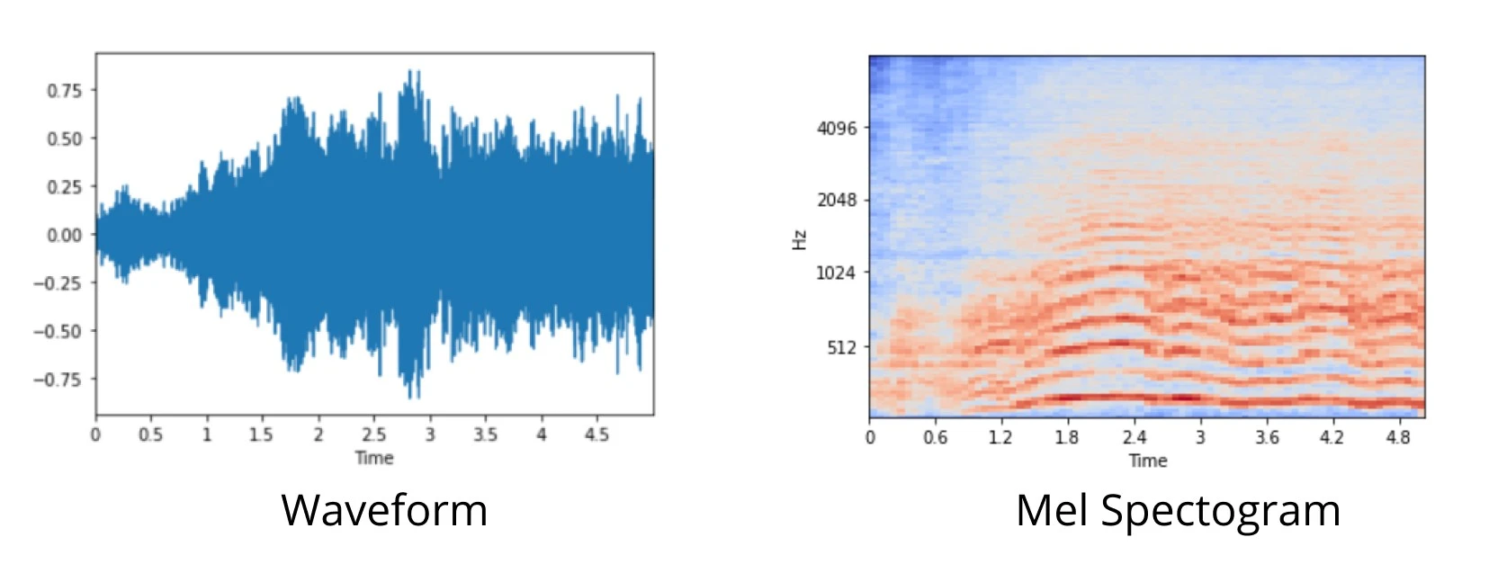
Waveform and Mel Spectogram

A waveform is an amplitude measurement put in a time series. There are many disadvantages to analyze the waveform, the data is big and messy, and the machine learning model doesn't perform well. The way around it is by analyzing the audio data and turn it into features, by analyzing it on the frequency domain (rather than amplitude) using math. In our experiment, we are using the Mel Spectrogram feature, this feature basically summarizes the waveform into a set of coefficients used in Mel Spectrogram and can be plotted like the image above. Using Mel Spectrogram which has less size than the actual waveform, we can train our model faster and get better performance too.

There are other features that we can extract from a waveform, like normal Spectrogram, MFCC, and many else. Here is a reference you can use to learn more about what is sound and how it is digitized.

Machine Learning Model

The most common approach use features like Mel Spectrogram and MFCC, but how about the model? Unexpectedly, the common CNN model used on image classification actually performs well on this data and has been a popularly used approach to classify audio.

In this project, we use the VGG16 model as our baseline. VGG16 is a popular CNN model used on image classification, the model achieves 92.7% top-5 test accuracy in ImageNet, which is a dataset of over 14 million images belonging to 1000 classes. VGG16 is consisted of 16 layers, with over 140M parameters and a size of 533MB. This makes training and deploying the model a tiresome task.

Our team did a modification to the model quite similar to this paper. Our augmented model has only 1M parameters, with a size of 15MB. The modification on the paper made are as follows :

1. Adding a Batch Normalization layer following each convolutional layer. Batch Normalization allows much higher learning rates and is less sensitive to initialization.
2. A global pooling layer replaces a flattened layer. Adding the global pooling layer not only helps filter the features but also makes the network adapt to different sizes of input spectrograms.
3. The 4096-unit FC layers are reduced to 256-unit FC layers.

Along with our modification as follows :

1. Adding dropout layer following each convolutional block.
2. Reducing the convolutional block from 4 to 3 blocks.

Our final model can be seen here.

Preprocessing and Training

After the model, there comes the preprocessing. The data we are using comes from 3 different sources and they have different characteristics too.

1. ESC-50; we are using the chainsaw and crackling fire sound from this dataset, all the audio data is 5 seconds long, with only 40 recordings for each class.
2. Urbansound5k; we are using the gunshot sound from this dataset, there are 374 recordings and the length varies from 1 to 4 seconds.
3. Google Audioset; all 3 classes exist here, the dataset itself is a list of associated YouTube ID, start time, end time, and class labels in a CSV file. To use the dataset as audio data, we need to download the recordings from youtube using a script that I have modified here.

To train the model, we need to have the same dimension of audio data, since we have various length of data, we decided to use only 2 seconds of recordings at a time. To get such data, we have to do some preprocessing.

1. ESC-50, we use a shifting windowing to trim 4 clips of 2 seconds from the original clip, totaling 40x4 = 160 clips for the 2 classes.
2. Urbansound5k, we are padding the recording with a length less than 2 seconds, and trimming the one with a length of more than 2 seconds.
3. The script to extract audio from youtube will download 10 seconds recordings. Using shifting windowing we will get 9 clips of 2 seconds from the original clip.

In our experiment, we are using 320 clips for each classes. The data which is still in the waveform then will be processed into Mel Spectrogram and shuffled into the train and validation dataset.

Training our model from scratch, the model got stopped by the callback after 15 epochs with results below.

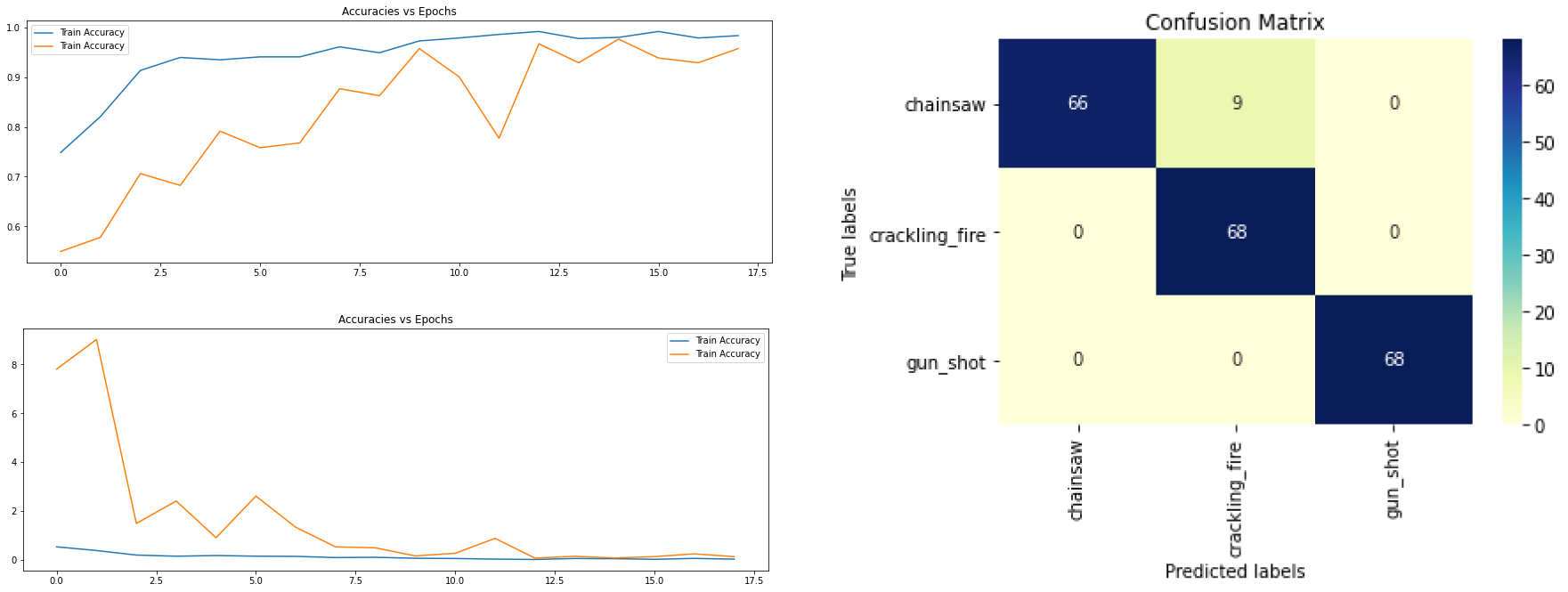
Accuracy & Loss History and Confusion Matrix

From the confusion matrix, we could see the model perform quite nicely for all 3 classes.

Inference / Predicting

We are using 2 seconds audio to train our model, but how do we analyze audio that has a different length or even through streaming? You could actually pass the whole audio data to the model, that is because the model could use any input size, but this method will perform worse than other methods. Another way to do it is by predicting a window of n seconds audio, and shifting it 1 second at a time, this method really works well but comes at a price, the computational needed will be huge.

What our team proposed is by reducing the noise from an audio clip, we could separate/highlight/isolate the target sounds that we want to hear. The target sounds will have a set of intervals, and the model will predict each highlighted clip separately. You can see the illustration of the method in the image below. After reducing the noise, the output results into 5 highlighted clips.

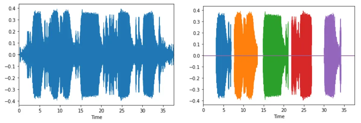
Before and After Highlighting the Sounds

Conclusion

There are still many aspects that could be improved, especially researching different model architecture, using a better dataset, and using a different audio feature like MFCC. Feel free to ask questions and using my Kaggle notebook as a reference, I hope my work on this project could help someone else in researching this topic.